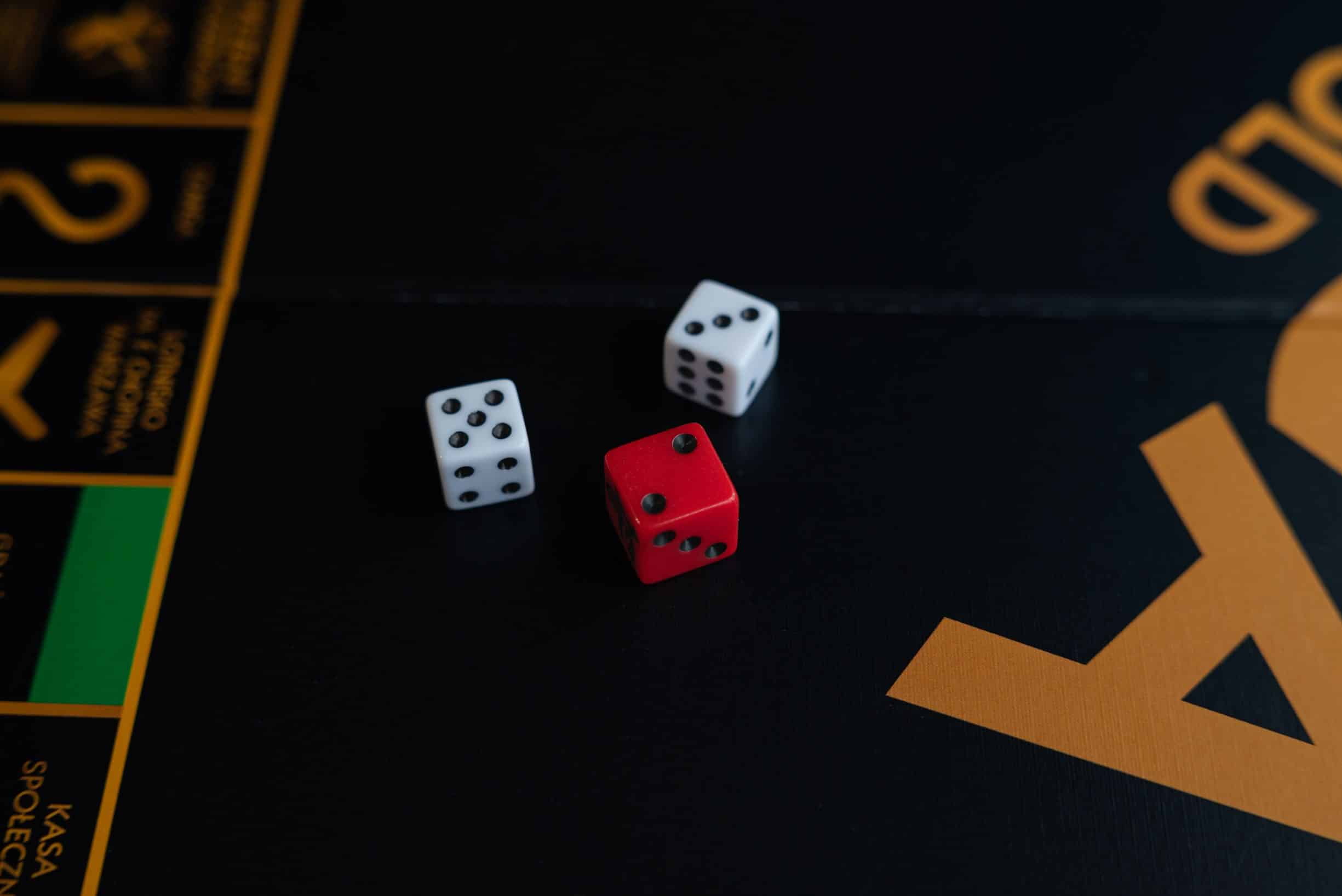
Elementary Probability Theory Made Easy for Discrete Mathematics Exam

Welcome, my dear students! Today we are going to learn about Elementary Probability Theory. I know many of you feel worried when you hear the word “probability,” but I promise you, if you follow my steps, it will become one of the easiest topics in your Discrete Mathematics course. So, let us begin together!

1. Sample Space and Events

Before we can talk about probability, we need to understand what we are measuring. Every probability problem starts with an experiment — an action whose result we cannot predict with certainty.

Definition: The sample space $S$ of an experiment is the set of all possible outcomes of that experiment.

An event $E$ is a subset of the sample space. It is a collection of one or more outcomes that we are interested in.

Let me give you a clear example. Suppose our experiment is rolling one fair die. What are all the possible outcomes?

Experiment: Roll one dieSample Space S = {1, 2, 3, 4, 5, 6}Event A: “Roll an even number” A = {2, 4, 6}Event B: “Roll a number greater than 4” B = {5, 6}

See how simple it is? The sample space is just a list of everything that CAN happen. An event is just picking the outcomes we care about from that list.

Types of Events You Must Know

Simple event (Elementary event): An event with only one outcome. For example, “rolling a 3” is $\{3\}$.

Impossible event: An event with no outcomes. Written as $\emptyset$ (empty set). For example, “rolling a 7 on a standard die” is impossible.

Certain event: An event that includes all outcomes. This is the sample space $S$ itself. For example, “rolling a number between 1 and 6” is certain.

Complement of an event: The complement of event $A$, written as $\overline{A}$ or $A^c$, is the set of all outcomes in $S$ that are NOT in $A$.

If S = {1, 2, 3, 4, 5, 6} and A = {2, 4, 6}Then A^c = {1, 3, 5} (all the odd numbers)Notice: A and A^c together give the full S Notice: A and A^c have NO common elements

Union of events ($A \cup B$): All outcomes that are in $A$ OR in $B$ (or both).

Intersection of events ($A \cap B$): All outcomes that are in $A$ AND in $B$ at the same time.

Mutually exclusive (Disjoint) events: Two events $A$ and $B$ are mutually exclusive if $A \cap B = \emptyset$. They cannot happen at the same time.

Worked Example 1: Working with Events

Problem: A fair die is rolled. Let $A = \{1, 2, 3\}$ and $B = \{3, 4, 5\}$. Find $A \cup B$, $A \cap B$, and $A^c$.

Solution: The sample space is $S = \{1, 2, 3, 4, 5, 6\}$.

$A \cup B = \{1, 2, 3, 4, 5\}$ (everything in A or B — note 3 appears only once)
$A \cap B = \{3\}$ (only 3 is in BOTH sets)
$A^c = \{4, 5, 6\}$ (everything in S that is NOT in A)

Important Exam Note: When writing a sample space, always make sure your outcomes are mutually exclusive (no overlap) and exhaustive (cover everything). For example, when flipping two coins, write $\{HH, HT, TH, TT\}$, NOT $\{0H, 1H, 2H\}$ unless the problem specifically asks for that format.

Practice Question 1 (MCQ): Two fair coins are tossed. The sample space is:
A) $\{H, T\}$
B) $\{HH, HT, TT\}$
C) $\{HH, HT, TH, TT\}$
D) $\{0, 1, 2\}$

Answer: C. When two coins are tossed, each coin can land Heads (H) or Tails (T). We must list ALL possible combinations for BOTH coins. Option A only shows one coin. Option B misses the outcome $TH$ (first coin tails, second coin heads) — remember that $HT$ and $TH$ are different outcomes! Option D shows the number of heads, which is a different way to describe outcomes but is not the full sample space listing.

Practice Question 2 (True/False): If event $A$ and event $B$ are mutually exclusive, then $A \cap B = S$.

Answer: False. If $A$ and $B$ are mutually exclusive (disjoint), then $A \cap B = \emptyset$ (the empty set), NOT $S$. They have NO outcomes in common. $A \cap B = S$ would mean they share ALL outcomes, which is the opposite of mutually exclusive.

Practice Question 3 (Fill in the Blank): A single card is drawn from a standard 52-card deck. The event “drawing a King” has ______ outcome(s) in the sample space.

Answer: 4. There are 4 Kings in a standard deck: King of Hearts, King of Diamonds, King of Clubs, and King of Spades. So the event “drawing a King” = $\{K\heartsuit, K\diamondsuit, K\clubsuit, K\spadesuit\}$, which contains 4 outcomes.

2. Probability of an Event

Now that we know what events are, let us learn how to measure how likely they are to happen. That measurement is called probability.

Definition (Equally Likely Outcomes): If all outcomes in a finite sample space $S$ are equally likely, then the probability of an event $A$ is:
\[ P(A) = \frac{|A|}{|S|} = \frac{\text{number of outcomes in } A}{\text{number of outcomes in } S} \]

This is the most basic and most frequently used formula in elementary probability. Let me show you how to use it.

Worked Example 2: Basic Probability

Problem: A fair die is rolled. Find the probability of getting an even number.

Solution: The sample space $S = \{1, 2, 3, 4, 5, 6\}$, so $|S| = 6$.
The event “even number” is $A = \{2, 4, 6\}$, so $|A| = 3$.
\[ P(A) = \frac{3}{6} = \frac{1}{2} \]

Worked Example 3: Card Problem

Problem: One card is drawn from a standard 52-card deck. Find the probability that it is a face card (Jack, Queen, or King).

Solution: $|S| = 52$ (total cards).
Each suit (Hearts, Diamonds, Clubs, Spades) has 3 face cards (J, Q, K). With 4 suits, total face cards $= 3 \times 4 = 12$.
\[ P(\text{Face card}) = \frac{12}{52} = \frac{3}{13} \]

Fundamental Rules of Probability

Now let me teach you the rules that apply to ALL probability problems, not just equally likely ones.

Rules to Remember for Exam:

Rule 1 (Range): For any event $A$: $\mathbf{0 \leq P(A) \leq 1}$
– $P(A) = 0$ means $A$ is impossible
– $P(A) = 1$ means $A$ is certain

Rule 2 (Certain event): $\mathbf{P(S) = 1}$

Rule 3 (Impossible event): $\mathbf{P(\emptyset) = 0}$

Rule 4 (Complement rule): $\mathbf{P(A^c) = 1 – P(A)}$
This is VERY useful when it is easier to find the probability of what you do NOT want.

Rule 5 (Addition rule): $\mathbf{P(A \cup B) = P(A) + P(B) – P(A \cap B)}$

Rule 6 (Mutually exclusive): If $A$ and $B$ are mutually exclusive: $\mathbf{P(A \cup B) = P(A) + P(B)}$
(Because $P(A \cap B) = 0$)

Worked Example 4: Using the Complement Rule

Problem: A fair die is rolled 4 times. What is the probability of getting at least one 6?

Solution: “At least one 6” means 1 or 2 or 3 or 4 sixes. Calculating this directly would be long. Instead, let us use the complement rule!

The complement of “at least one 6” is “no sixes at all” (getting 6 is false every time).

\begin{aligned} P(\text{no 6 in one roll}) &= \frac{5}{6} \\ P(\text{no 6 in four rolls}) &= \left(\frac{5}{6}\right)^4 = \frac{625}{1296} \\ P(\text{at least one 6}) &= 1 – \frac{625}{1296} = \frac{671}{1296} \end{aligned}

Exam Tip: Whenever you see the words “at least one”, immediately think of the complement rule. It will save you so much time! The complement of “at least one” is “none.”

Worked Example 5: Using the Addition Rule

Problem: A card is drawn from a standard deck. Find the probability of drawing a King OR a Heart.

Solution: Let $A =$ “drawing a King” and $B =$ “drawing a Heart.”
$P(A) = \frac{4}{52}$ (4 Kings)
$P(B) = \frac{13}{52}$ (13 Hearts)
$P(A \cap B) = \frac{1}{52}$ (the King of Hearts — it is BOTH a King and a Heart)

P(A \cup B) = \frac{4}{52} + \frac{13}{52} – \frac{1}{52} = \frac{16}{52} = \frac{4}{13}

Why subtract? Because the King of Hearts was counted in BOTH $P(A)$ and $P(B)$. If we just add, we count it twice. We must subtract the overlap once.

Practice Question 4 (MCQ): The probability of event $A$ is 0.7. What is $P(A^c)$?
A) 0.7
B) 0.3
C) 1.7
D) -0.7

Answer: B. By the complement rule, $P(A^c) = 1 – P(A) = 1 – 0.7 = 0.3$. This is one of the simplest yet most useful formulas. Also note that probabilities can never be negative (option D) or greater than 1 (option C).

Practice Question 5 (MCQ): If $P(A) = 0.4$, $P(B) = 0.5$, and $P(A \cap B) = 0.1$, what is $P(A \cup B)$?
A) 0.9
B) 0.8
C) 0.2
D) 1.0

Answer: B. Using the addition rule: $P(A \cup B) = P(A) + P(B) – P(A \cap B) = 0.4 + 0.5 – 0.1 = 0.8$. If you forgot to subtract the intersection, you would get 0.9 (option A) — a very common mistake!

Practice Question 6 (Short Answer): Can the probability of an event be 1.05? Explain why or why not.

Answer: No, the probability of any event must satisfy $0 \leq P(A) \leq 1$. A probability of 1.05 is greater than 1, which is impossible. The maximum probability is 1 (for a certain event). If you ever get a probability greater than 1 in your calculation, you made a mistake somewhere.

3. Conditional Probability

Now, let me ask you a question. Suppose I tell you that I drew a card and it is a Heart. Now, what is the probability that it is also a King? Notice that I gave you extra information — I told you the card is a Heart. This changes the problem! This is what conditional probability is all about.

Definition: The conditional probability of event $A$ given that event $B$ has already occurred is:
\[ P(A \mid B) = \frac{P(A \cap B)}{P(B)} \]
Read this as “the probability of $A$ given $B$.”

In simple words: “Given that $B$ has happened, what is the chance that $A$ also happens?” We divide the probability of BOTH happening by the probability of $B$.

Worked Example 6: Conditional Probability with Cards

Problem: A card is drawn from a standard deck. Given that the card is a Heart, find the probability that it is a King.

Solution: Let $A =$ “card is a King” and $B =$ “card is a Heart.”
We need $P(A \mid B) = \frac{P(A \cap B)}{P(B)}$

$P(A \cap B) = P(\text{King of Hearts}) = \frac{1}{52}$
$P(B) = P(\text{Heart}) = \frac{13}{52}$

P(A \mid B) = \frac{1/52}{13/52} = \frac{1}{13}

Intuitive check: If we KNOW the card is a Heart, we are now choosing from only 13 cards (the Hearts). Among these 13 Hearts, only 1 is a King. So $1/13$ makes perfect sense!

Intuitive Way to Think About Conditional Probability:
When you are told that event $B$ has happened, shrink your sample space from $S$ to just $B$. Now count how many outcomes in $B$ also satisfy $A$.
\[ P(A \mid B) = \frac{|A \cap B|}{|B|} \]
This is often easier to use than the formula with probabilities!

Worked Example 7: Conditional Probability with Dice

Problem: Two fair dice are rolled. Given that the sum is 8, what is the probability that at least one die shows a 3?

Solution: First, let me list all outcomes where the sum is 8 (this is our new “sample space” given $B$):

Sum = 8 outcomes (ordered pairs): (2,6), (3,5), (4,4), (5,3), (6,2) Total: |B| = 5

Now, which of these have at least one 3?

(3,5) — has a 3 ✓ (5,3) — has a 3 ✓ Count: |A ∩ B| = 2

P(A \mid B) = \frac{|A \cap B|}{|B|} = \frac{2}{5}

Multiplication Rule

From the definition of conditional probability, we can derive a very useful formula:

Multiplication Rule:
\[ P(A \cap B) = P(A) \cdot P(B \mid A) = P(B) \cdot P(A \mid B) \]
This rule is used when you need to find the probability that TWO events BOTH happen.

Worked Example 8: Using the Multiplication Rule

Problem: A bag contains 5 red and 3 blue balls. Two balls are drawn WITHOUT replacement. Find the probability that both are red.

Solution: Let $R_1 =$ “first ball is red” and $R_2 =$ “second ball is red.”

\begin{aligned} P(R_1) &= \frac{5}{8} \quad \text{(5 red out of 8 total)} \\ P(R_2 \mid R_1) &= \frac{4}{7} \quad \text{(4 red left out of 7 total, since one red was removed)} \\ P(R_1 \cap R_2) &= P(R_1) \cdot P(R_2 \mid R_1) = \frac{5}{8} \cdot \frac{4}{7} = \frac{20}{56} = \frac{5}{14} \end{aligned}

Exam Tip — “Without Replacement”: Whenever a problem says “without replacement,” you MUST use conditional probability for the second draw because the sample space changes! If it says “with replacement,” the probabilities stay the same for each draw.

Practice Question 7 (MCQ): If $P(A) = 0.6$, $P(B) = 0.4$, and $P(A \cap B) = 0.24$, what is $P(A \mid B)$?
A) 0.6
B) 0.4
C) 0.24
D) 0.96

Answer: A. $P(A \mid B) = \frac{P(A \cap B)}{P(B)} = \frac{0.24}{0.4} = 0.6$. Interestingly, this equals $P(A)$, which means $A$ and $B$ are independent (more on that soon!). But the calculation is just the formula — divide the intersection by the given event.

Practice Question 8 (True/False): $P(A \mid B)$ can be greater than $P(A)$.

Answer: True. Knowing that $B$ occurred can INCREASE the probability of $A$. For example, if $A =$ “card is a King” and $B =$ “card is a face card,” then $P(A) = 4/52 \approx 0.077$ but $P(A \mid B) = 4/12 \approx 0.333$. The conditional probability is much higher because knowing the card is a face card narrows down the possibilities.

Practice Question 9 (Fill in the Blank): Two cards are drawn from a deck without replacement. The probability that the second card is an Ace given that the first card is an Ace is ______.

Answer: 3/51 = 1/17. After drawing one Ace, there are 51 cards left and only 3 Aces remaining. So $P(\text{second Ace} \mid \text{first Ace}) = 3/51 = 1/17$. The key is recognizing that “without replacement” changes the count.

4. Independent Events

Now let me ask you: if I flip a coin and get Heads, does that change the probability of getting Heads on the NEXT flip? No! The coin does not remember what happened before. This idea leads us to independent events.

Definition: Two events $A$ and $B$ are independent if the occurrence of one does NOT affect the probability of the other. Mathematically:
\[ P(A \mid B) = P(A) \quad \text{or equivalently} \quad P(B \mid A) = P(B) \]

Most useful test for independence:
\[ P(A \cap B) = P(A) \cdot P(B) \]
If this equality holds, $A$ and $B$ are independent. If it does NOT hold, they are dependent.

Biggest Mistake Students Make: Do NOT confuse “independent” with “mutually exclusive”! They are completely different ideas:
– Mutually exclusive: $A \cap B = \emptyset$ (they cannot happen together)
– Independent: $P(A \cap B) = P(A) \cdot P(B)$ (one does not affect the other)

In fact, if $A$ and $B$ are both mutually exclusive AND both have positive probability, they are ALWAYS dependent (not independent)! Because if they are mutually exclusive, $P(A \cap B) = 0$, but $P(A) \cdot P(B) > 0$, so the equality fails.

Worked Example 9: Checking Independence

Problem: A fair die is rolled. Let $A = \{1, 2, 3, 4\}$ (roll is at most 4) and $B = \{2, 4, 6\}$ (roll is even). Are $A$ and $B$ independent?

Solution: Check if $P(A \cap B) = P(A) \cdot P(B)$.

$A \cap B = \{2, 4\}$, so $P(A \cap B) = \frac{2}{6} = \frac{1}{3}$
$P(A) = \frac{4}{6} = \frac{2}{3}$
$P(B) = \frac{3}{6} = \frac{1}{2}$
$P(A) \cdot P(B) = \frac{2}{3} \cdot \frac{1}{2} = \frac{1}{3}$

Since $\frac{1}{3} = \frac{1}{3}$, YES, $A$ and $B$ are independent!

Worked Example 10: Independent vs Dependent

Problem: A card is drawn from a standard deck. Let $A =$ “card is a King” and $B =$ “card is a Heart.” Are they independent?

Solution: Check: $P(A \cap B) = \frac{1}{52}$. And $P(A) \cdot P(B) = \frac{4}{52} \cdot \frac{13}{52} = \frac{52}{2704} = \frac{1}{52}$.
Since $\frac{1}{52} = \frac{1}{52}$, they ARE independent! This may surprise you, but it is true — knowing a card is a Heart does not change the probability of it being a King (it stays 1/13).

Worked Example 11: Using Independence to Find Joint Probability

Problem: A fair coin is flipped 3 times. What is the probability of getting Heads on all three flips?

Solution: Each flip is independent of the others. Let $H_1, H_2, H_3$ be the events “Heads on flip 1, 2, 3.”

P(H_1 \cap H_2 \cap H_3) = P(H_1) \cdot P(H_2) \cdot P(H_3) = \frac{1}{2} \cdot \frac{1}{2} \cdot \frac{1}{2} = \frac{1}{8}

This is why we often say: for independent events, just multiply the probabilities!

Summary of When to Multiply vs Add:
– AND (both events happen, $\cap$): Multiply probabilities (use multiplication rule; if independent, just multiply directly)
– OR (at least one happens, $\cup$): Add probabilities (use addition rule, but remember to subtract the overlap)

Practice Question 10 (MCQ): If $A$ and $B$ are independent events with $P(A) = 0.3$ and $P(B) = 0.5$, what is $P(A \cap B)$?
A) 0.8
B) 0.15
C) 0.2
D) 0.05

Answer: B. For independent events, $P(A \cap B) = P(A) \cdot P(B) = 0.3 \times 0.5 = 0.15$. Option A is the sum (wrong operation). Option C would be if you averaged them. Option D has no basis.

Practice Question 11 (True/False): If two events are mutually exclusive, they must be independent.

Answer: False. This is the most common confusion! If two events are mutually exclusive and both have positive probability, they are DEPENDENT. Here is why: if $A$ happens, you know for sure that $B$ did NOT happen (since they cannot co-occur). So knowing $A$ occurred changes the probability of $B$ to 0, which means they are dependent. Mutually exclusive $\neq$ independent!

Practice Question 12 (MCQ): Two events $A$ and $B$ satisfy $P(A) = 0.2$, $P(B) = 0.6$, and $P(A \cap B) = 0.15$. Are $A$ and $B$ independent?
A) Yes, because $P(A) + P(B) < 1$
B) No, because $P(A) \cdot P(B) = 0.12 \neq 0.15$
C) Yes, because $P(A \cap B) > 0$
D) Cannot be determined

Answer: B. The test for independence is: does $P(A \cap B) = P(A) \cdot P(B)$? Here, $P(A) \cdot P(B) = 0.2 \times 0.6 = 0.12$, but $P(A \cap B) = 0.15$. Since $0.12 \neq 0.15$, the events are NOT independent. Always use this multiplication test — it is the definitive check.

5. Random Variables and Expectation

We have now reached the last major topic. A random variable is a way to turn the outcomes of an experiment into numbers. Instead of saying “we got Heads,” we assign a number to it.

Definition: A random variable is a function that assigns a numerical value to each outcome in the sample space.

We use capital letters like $X, Y, Z$ for random variables, and lowercase letters like $x, y, z$ for their specific values.

Discrete random variable: Takes a finite or countable number of values (like 0, 1, 2, 3, …).
Continuous random variable: Takes values in a continuous range (like any number between 0 and 1). In this course, we focus on discrete random variables.

Worked Example 12: Defining a Random Variable

Problem: Three coins are tossed. Let $X$ = “number of Heads obtained.” Find the possible values of $X$ and the probability of each value.

Solution: Sample space: $\{HHH, HHT, HTH, THH, HTT, THT, TTH, TTT\}$ (8 outcomes, all equally likely).

Value of $X$	Outcomes	Count	$P(X = x)$
0	$TTT$	1	$1/8$
1	$HTT, THT, TTH$	3	$3/8$
2	$HHT, HTH, THH$	3	$3/8$
3	$HHH$	1	$1/8$

This table is called the probability distribution of $X$. Notice that the probabilities add up to 1: $\frac{1}{8} + \frac{3}{8} + \frac{3}{8} + \frac{1}{8} = 1$.

Expected Value (Expectation)

Definition: The expected value (or mean or expectation) of a discrete random variable $X$ is:
\[ E(X) = \sum x \cdot P(X = x) \]
You multiply each value by its probability and add up all the results.

Think of it as a weighted average — values with higher probability “weigh” more.

Worked Example 13: Calculating Expected Value

Problem: Find $E(X)$ for the coin-tossing random variable from Example 12.

Solution:

\begin{aligned} E(X) &= 0 \cdot \frac{1}{8} + 1 \cdot \frac{3}{8} + 2 \cdot \frac{3}{8} + 3 \cdot \frac{1}{8} \\ &= 0 + \frac{3}{8} + \frac{6}{8} + \frac{3}{8} \\ &= \frac{12}{8} = \frac{3}{2} = 1.5 \end{aligned}

So the expected number of Heads when flipping 3 fair coins is 1.5. This makes sense — on average, half the flips are Heads, and $3/2 = 1.5$.

Important: The expected value does NOT have to be one of the possible values! Here, $X$ can only be 0, 1, 2, or 3, but $E(X) = 1.5$. The expected value is an AVERAGE, not a prediction of a single outcome.

Worked Example 14: Expected Value of a Game

Problem: You pay $3 to play a game. A fair die is rolled. If you roll a 6, you win $10. Otherwise, you win nothing. What is your expected gain (or loss)?

Solution: Let $X$ = net gain. We need to account for the $3 cost.

Roll a 6 (probability $1/6$): you receive $10 but paid $3, so net gain = $10 – 3 = 7$
Roll 1-5 (probability $5/6$): you receive $0 but paid $3, so net gain = $0 – 3 = -3$

E(X) = 7 \cdot \frac{1}{6} + (-3) \cdot \frac{5}{6} = \frac{7}{6} – \frac{15}{6} = \frac{-8}{6} = -\frac{4}{3} \approx -1.33

Your expected gain is about -$1.33. This means on average, you lose about $1.33 per game. This is a fair game question — if the expected value is negative, the game favors the house!

Properties of Expected Value

Useful Properties for Exam:

1. $E(c) = c$ for any constant $c$
2. $E(cX) = c \cdot E(X)$ for any constant $c$
3. $E(X + Y) = E(X) + E(Y)$ even if $X$ and $Y$ are NOT independent!
4. If $X$ and $Y$ are independent, then $E(XY) = E(X) \cdot E(Y)$

Property 3 is very powerful — you do NOT need independence to add expectations!

Worked Example 15: Linearity of Expectation

Problem: A fair die is rolled 10 times. Let $X$ = total sum of all rolls. Find $E(X)$.

Solution: Let $X_i$ = value of the $i$-th roll. Then $X = X_1 + X_2 + \cdots + X_{10}$.

For one fair die: $E(X_i) = \frac{1+2+3+4+5+6}{6} = \frac{21}{6} = 3.5$

By linearity (Property 3):

E(X) = E(X_1) + E(X_2) + \cdots + E(X_{10}) = 10 \times 3.5 = 35

We did NOT need to find the distribution of the sum (which would be very complex). We just used linearity of expectation!

Practice Question 13 (MCQ): A random variable $X$ has the distribution: $P(X=0)=0.2$, $P(X=1)=0.5$, $P(X=2)=0.3$. What is $E(X)$?
A) 1.0
B) 1.1
C) 1.5
D) 2.0

Answer: B. $E(X) = 0(0.2) + 1(0.5) + 2(0.3) = 0 + 0.5 + 0.6 = 1.1$. Just multiply each value by its probability and add.

Practice Question 14 (True/False): If $E(X) = 3$, then the most likely value of $X$ is 3.

Answer: False. The expected value is a weighted average, not the most likely value (which is called the mode). For example, if $X = 0$ with probability 0.9 and $X = 30$ with probability 0.1, then $E(X) = 0(0.9) + 30(0.1) = 3$. The expected value is 3, but the most likely value is 0!

Practice Question 15 (Short Answer): A game costs $2 to play. You draw a card from a standard deck. If it is an Ace, you win $15. Otherwise, you win nothing. Is this game fair? (A fair game has expected net gain = 0.)

Answer: Let $X$ = net gain. $P(\text{Ace}) = 4/52 = 1/13$, so net gain $= 15 – 2 = 13$. $P(\text{not Ace}) = 12/13$, so net gain $= 0 – 2 = -2$.
$E(X) = 13 \cdot \frac{1}{13} + (-2) \cdot \frac{12}{13} = 1 – \frac{24}{13} = \frac{13 – 24}{13} = \frac{-11}{13} \approx -0.85$
Since $E(X) \neq 0$ (it is negative), the game is NOT fair. It favors the house — you lose about $0.85 per game on average.

6. Quick Summary of All Key Formulas

Concept	Formula
Basic probability	$P(A) = \frac{\|A\|}{\|S\|}$
Complement rule	$P(A^c) = 1 – P(A)$
Addition rule	$P(A \cup B) = P(A) + P(B) – P(A \cap B)$
Mutually exclusive	$P(A \cup B) = P(A) + P(B)$
Conditional probability	$P(A \mid B) = \frac{P(A \cap B)}{P(B)}$
Multiplication rule	$P(A \cap B) = P(A) \cdot P(B \mid A)$
Independence test	$P(A \cap B) = P(A) \cdot P(B)$
Expected value	$E(X) = \sum x \cdot P(X=x)$
Linearity	$E(X+Y) = E(X) + E(Y)$

Final Exam Tips:
1. Always define your events clearly with letters (like $A, B$) before starting.
2. For “at least one” problems, use the complement rule immediately.
3. For “without replacement” problems, use conditional probability.
4. To check independence, always multiply $P(A) \cdot P(B)$ and compare with $P(A \cap B)$.
5. For expected value, make a table of values and probabilities, then multiply and add.
6. Never forget: probability is always between 0 and 1, and all probabilities in a distribution must sum to 1.

Challenge Conceptual Exam Questions

These questions test your deep understanding. Take your time and think carefully!

Multiple Choice Questions

Q1. If $P(A \cup B) = 0.8$, $P(A \cap B) = 0.2$, and $P(A) = 0.5$, what is $P(B)$?
A) 0.3
B) 0.5
C) 0.6
D) 0.1

Answer: B. From the addition rule: $P(A \cup B) = P(A) + P(B) – P(A \cap B)$. Substituting: $0.8 = 0.5 + P(B) – 0.2$, so $0.8 = 0.3 + P(B)$, giving $P(B) = 0.5$. The key is to rearrange the addition rule correctly.

Q2. Events $A$ and $B$ are independent. $P(A) = 0.4$ and $P(B) = 0.3$. What is $P(A \mid B)$?
A) 0.12
B) 0.4
C) 0.7
D) 0.3

Answer: B. By definition of independence, $P(A \mid B) = P(A) = 0.4$. This is the whole point of independence — knowing $B$ occurred does not change the probability of $A$. Option A ($0.12$) is $P(A \cap B)$, not $P(A \mid B)$. Do not confuse these!

Q3. A random variable $X$ has $E(X) = 5$. What is $E(3X + 2)$?
A) 15
B) 17
C) 21
D) 7

Answer: B. Using the properties: $E(3X + 2) = E(3X) + E(2) = 3 \cdot E(X) + 2 = 3(5) + 2 = 17$. Remember: $E(cX) = c \cdot E(X)$ and $E(\text{constant}) = \text{constant}$.

Q4. Two dice are rolled. What is the probability that the sum is 7 OR at least one die shows a 6?
A) $\frac{7}{12}$
B) $\frac{5}{12}$
C) $\frac{1}{2}$
D) $\frac{2}{3}$

Answer: A. Let $A =$ “sum is 7” and $B =$ “at least one 6.”
$A = \{(1,6),(2,5),(3,4),(4,3),(5,2),(6,1)\}$, so $P(A) = 6/36$.
$B = $ all outcomes with at least one 6. There are $6 + 6 – 1 = 11$ such outcomes, so $P(B) = 11/36$.
$A \cap B = \{(1,6),(6,1)\}$, so $P(A \cap B) = 2/36$.
$P(A \cup B) = 6/36 + 11/36 – 2/36 = 15/36 = 5/12$… Wait, that gives option B. Let me recount $B$: outcomes with a 6 are $(6,1),(6,2),(6,3),(6,4),(6,5),(6,6),(1,6),(2,6),(3,6),(4,6),(5,6) = 11$. So $P(B) = 11/36$. Then $P(A \cup B) = 6/36 + 11/36 – 2/36 = 15/36 = 5/12$.
Correction: Answer is B ($5/12$). I made an arithmetic error in my initial check. Always verify carefully!

True / False Questions

Q5. If $P(A \mid B) = P(B \mid A)$, then $P(A) = P(B)$.

Answer: True. If $P(A \mid B) = P(B \mid A)$, then $\frac{P(A \cap B)}{P(B)} = \frac{P(A \cap B)}{P(A)}$. Assuming $P(A \cap B) \neq 0$, we can cancel it to get $\frac{1}{P(B)} = \frac{1}{P(A)}$, which means $P(A) = P(B)$. This is a nice theoretical result!

Q6. If $E(X) = 0$, then $X$ must always equal 0.

Answer: False. $E(X) = 0$ only means the weighted average is 0. For example, $X = -1$ with probability 0.5 and $X = 1$ with probability 0.5 gives $E(X) = -0.5 + 0.5 = 0$, but $X$ is never actually 0.

Q7. If $A$ and $B$ are independent, then $A^c$ and $B^c$ are also independent.

Answer: True. This is a theorem. If $A$ and $B$ are independent, then $P(A^c \cap B^c) = 1 – P(A) – P(B) + P(A)P(B) = (1-P(A))(1-P(B)) = P(A^c) \cdot P(B^c)$. So $A^c$ and $B^c$ satisfy the independence condition. Similarly, $A$ and $B^c$ are independent, and $A^c$ and $B$ are independent.

Q8. For any two events $A$ and $B$, $P(A \cap B) \leq P(A)$.

Answer: True. Since $A \cap B \subseteq A$, the probability of the intersection cannot exceed the probability of $A$. Think of it as: the chance of BOTH $A$ and $B$ happening cannot be greater than the chance of just $A$ happening. Similarly, $P(A \cap B) \leq P(B)$.

Fill in the Blank Questions

Q9. If $P(A) = 0.6$ and $P(A \cap B) = 0.3$, then the largest possible value of $P(B)$ is ______.

Answer: 1. Since $P(A \cap B) \leq P(B)$ always, we know $P(B) \geq 0.3$. But what is the MAXIMUM? It can be at most 1 (since no probability exceeds 1). Can $P(B) = 1$? Yes, if $B = S$ (the entire sample space), then $P(B) = 1$ and $P(A \cap B) = P(A) = 0.6$… but we need $P(A \cap B) = 0.3$. If $P(B) = 1$, then $A \cap B = A$, so $P(A \cap B) = P(A) = 0.6 \neq 0.3$. So we need $P(B) \leq 1$ AND $P(A \cap B) \leq P(B)$, which gives $P(B) \geq 0.3$. Also, by the addition rule: $P(A \cup B) \leq 1$, so $P(A) + P(B) – P(A \cap B) \leq 1$, giving $0.6 + P(B) – 0.3 \leq 1$, so $P(B) \leq 0.7$. The largest possible value is 0.7.

Q10. A fair coin is flipped $n$ times. The expected number of Heads is ______.

Answer: $n/2$. Let $X_i = 1$ if the $i$-th flip is Heads, 0 otherwise. Then $E(X_i) = 1 \cdot \frac{1}{2} + 0 \cdot \frac{1}{2} = \frac{1}{2}$. Total Heads $X = X_1 + X_2 + \cdots + X_n$, so $E(X) = n \cdot \frac{1}{2} = \frac{n}{2}$. This uses linearity of expectation.

Q11. If $P(A) = 0.5$ and $P(B \mid A) = 0.4$, then $P(A \cap B) = $ ______.

Answer: 0.2. By the multiplication rule: $P(A \cap B) = P(A) \cdot P(B \mid A) = 0.5 \times 0.4 = 0.2$. This is a direct application of the formula — just multiply!

Short Answer / Workout Questions

Q12. A bag contains 4 red balls and 6 green balls. Three balls are drawn without replacement. Find the probability that all three are the same color.

Answer: “All same color” means either all red OR all green. These are mutually exclusive events.

$P(\text{all red}) = \frac{4}{10} \cdot \frac{3}{9} \cdot \frac{2}{8} = \frac{24}{720} = \frac{1}{30}$
$P(\text{all green}) = \frac{6}{10} \cdot \frac{5}{9} \cdot \frac{4}{8} = \frac{120}{720} = \frac{1}{6}$

$P(\text{all same color}) = \frac{1}{30} + \frac{1}{6} = \frac{1}{30} + \frac{5}{30} = \frac{6}{30} = \frac{1}{5}$

The key was recognizing “OR” and using the addition rule for mutually exclusive events, combined with the multiplication rule for each case.

Q13. A student knows 70% of the material. On a true/false test with 10 questions, if the student answers each question correctly when they know the material, and guesses (50% chance) when they do not, what is the expected number of correct answers?

Answer: For each question, let $X_i$ = 1 if correct, 0 if wrong.
$P(X_i = 1) = P(\text{knows}) \cdot 1 + P(\text{doesn’t know}) \cdot 0.5 = 0.7 \times 1 + 0.3 \times 0.5 = 0.7 + 0.15 = 0.85$
So $E(X_i) = 0.85$ for each question.
Total correct $X = X_1 + \cdots + X_{10}$, so $E(X) = 10 \times 0.85 = 8.5$.
The expected number of correct answers is 8.5.

Q14. Prove that if $A$ and $B$ are events with $P(A) > 0$ and $P(B) > 0$, and $A$ and $B$ are mutually exclusive, then they are dependent.

Answer: Since $A$ and $B$ are mutually exclusive, $A \cap B = \emptyset$, so $P(A \cap B) = 0$.

For independence, we would need $P(A \cap B) = P(A) \cdot P(B)$. But $P(A) \cdot P(B) > 0$ (since both probabilities are positive).

So $0 = P(A \cap B) \neq P(A) \cdot P(B) > 0$. The independence condition fails.

Therefore, $A$ and $B$ are dependent. Intuitively: if $A$ occurs, then $B$ cannot occur (they are mutually exclusive), so knowing $A$ happened changes $P(B)$ to 0, which proves dependence.

Q15. A box contains 3 defective and 7 good items. Items are drawn one by one without replacement until the first defective is found. Let $X$ = number of draws needed. Find the probability distribution of $X$ and $E(X)$.

Answer: $X$ can be 1, 2, 3, or 4 (if the first 3 are good, the 4th must be defective since there are only 7 good items… wait, there are 7 good items, so we could draw up to 8 good items before hitting a defective. Actually, the maximum value of $X$ is 8 — we could draw all 7 good items first, then the 8th draw must be defective).

Let me reconsider: $X$ is the position of the first defective. It can be 1, 2, …, 8.

$P(X=1) = \frac{3}{10}$ (first item is defective)
$P(X=2) = \frac{7}{10} \cdot \frac{3}{9} = \frac{21}{90} = \frac{7}{30}$ (first good, then defective)
$P(X=3) = \frac{7}{10} \cdot \frac{6}{9} \cdot \frac{3}{8} = \frac{126}{720} = \frac{7}{40}$
$P(X=4) = \frac{7}{10} \cdot \frac{6}{9} \cdot \frac{5}{8} \cdot \frac{3}{7} = \frac{630}{5040} = \frac{1}{8}$
…and so on. The pattern is $P(X=k) = \frac{\binom{7}{k-1}}{\binom{10}{k-1}} \cdot \frac{3}{10-(k-1)}$.

For $E(X)$, we could compute: $E(X) = 1 \cdot \frac{3}{10} + 2 \cdot \frac{7}{30} + 3 \cdot \frac{7}{40} + \cdots$ This requires computing all 8 terms. However, there is a clever shortcut: for sampling without replacement from $N$ items with $K$ defectives, $E(X) = \frac{N+1}{K+1} = \frac{11}{4} = 2.75$. So $E(X) = 2.75$.

Value of \(X\)	Outcomes	Count	\(P(X = x)\)
0	\(TTT\)	1	\(1/8\)
1	\(HTT, THT, TTH\)	3	\(3/8\)
2	\(HHT, HTH, THH\)	3	\(3/8\)
3	\(HHH\)	1	\(1/8\)